Payback analysis for the top mobile manipulator use cases
Why utilisation across stations is the make-or-break variable in every scenario
Utilisation is the business case
Every mobile manipulator payback model rests on a single lever: how much of the robot's available time is spent performing value-added work. A fixed arm parked at one machine can be cost-effective at 40–50 percent utilisation because it has no transit overhead. A mobile manipulator circulating between stations spends a real fraction of every cycle on navigation, docking, and re-localisation. If the tasks at each station are short relative to the transit overhead, the robot is expensive and slow compared to alternatives.
The utilisation equation for a mobile manipulator is:
Productive time = Shift hours × (1 − transit fraction) × (1 − downtime fraction)
Where transit fraction includes not just movement but docking, re-localisation, and any battery charging that interrupts production. For typical indoor factory environments, transit fraction runs 15–30 percent; a poorly sited deployment can reach 40 percent and never recover.
This article works through three use cases — multi-station machine tending, lab and sample automation, and kitting/parts-to-line — showing where utilisation typically lands, what payback period looks like at different utilisation levels, and what operational choices determine which end of that range you hit.
Use case 1: Multi-station machine tending
What the task looks like
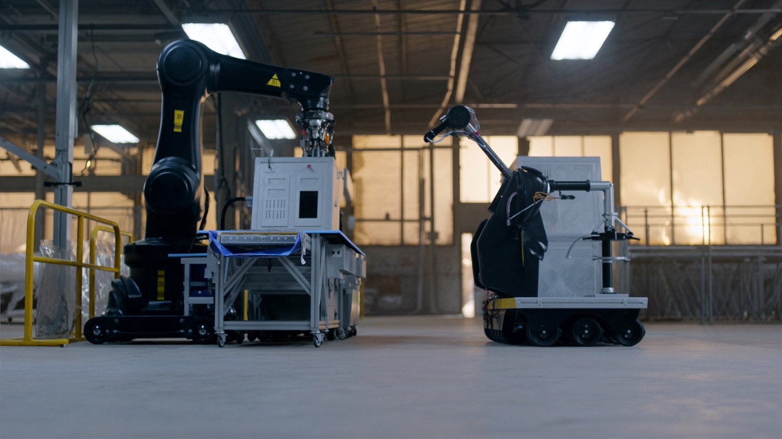
A mobile manipulator circulates between three to six CNC lathes, milling centres, or injection moulding presses. At each station, it opens a machine door, removes a finished part, loads a raw blank, and closes the door. Part tolerances are typically ±0.1–0.5 mm — achievable with fiducial re-localisation (see When a mobile manipulator beats a fixed arm). Cycle times per station visit range from 45 to 180 seconds depending on part complexity.
Platforms deployed in this pattern include the Robotnik RB-KAIROS+ (configured with a UR or equivalent cobot arm) and similar industrial mobile manipulation platforms from Asian manufacturers including Youibot's ARIS-CH.
Utilisation model
Assume a circuit of four machines, each with a 90-second part-load/unload cycle, 30-second navigation transit between adjacent machines, and 15-second re-localisation per station:
| Metric | Value |
|---|---|
| Per-station productive time | 90 s |
| Per-station overhead (transit + dock + re-localise) | 45 s |
| Per-station efficiency | 67% |
| Full circuit time (4 stations) | 540 s = 9 min |
| Shift hours utilised productively | ~65% |
| Battery charge interruption (45 min/8-hr shift) | −9% |
| Net productive utilisation | ~56% |
At 56 percent productive utilisation across four stations, the mobile manipulator is doing the work of roughly 2.2 dedicated fixed arms. If a single fixed arm serves one machine and requires one FTE to load/unload the others manually, the comparison shifts based on labour cost.
Payback at representative utilisation levels
Assumptions: hardware + integration capital $320,000; avoided labour cost $55,000/year per FTE; machine utilisation gain (eliminating wait time for human operators) valued at $30,000/year.
| Productive utilisation | Annualised value | Payback period |
|---|---|---|
| 40% (3 stations, light loads) | $55,000–$70,000 | 4.5–6 years |
| 55% (4 stations, standard cycle) | $85,000–$110,000 | 2.9–3.8 years |
| 70% (5–6 stations, optimised circuit) | $120,000–$150,000 | 2.1–2.7 years |
The 3–4 year payback at 55 percent utilisation is achievable but requires the circuit to be kept full. The most common failure mode: one machine goes into unplanned maintenance for a week, reducing the circuit to three stations and dropping utilisation to 40 percent. Over a year with several such events, average utilisation can fall below the threshold that justifies the capital.
Key operational rule: build the circuit for n+1 stations so that losing one station to maintenance still keeps utilisation above 50 percent.
Use case 2: Lab and sample automation
What the task looks like
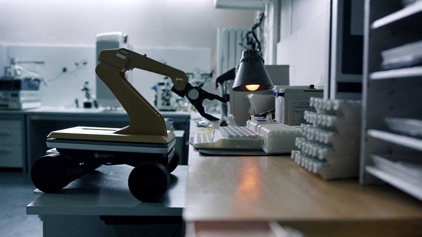
A mobile manipulator transports samples between benches, loads/unloads centrifuges, incubators, or analytical instruments, and places labelled vials into defined positions. Lab automation is a natural fit for mobile manipulation because: tolerances are moderate (±1–3 mm for most vial placements), payloads are light (typically <3 kg), floor layouts are dense and change with experiments, and human labour in labs is expensive.
Research-adjacent platforms like the University of Washington's Herb (herb) and Toyota's Human Support Robot (human-support-robot-1) pioneered this use case in academic settings. Commercial lab automation deployments have adopted dedicated mobile manipulation platforms and cobot-on-base configurations.
Why lab automation is a stronger use case than factory tending
Three structural differences make lab automation a more favourable environment for mobile manipulation:
Tolerance is more forgiving. A centrifuge rotor that accepts a 15 mm tube has ±3–5 mm of part placement clearance. A CNC lathe chuck does not. This means fiducial re-localisation — or even force-compliant insertion — can reliably achieve the required accuracy without elaborate docking infrastructure.
Labour cost is higher. Lab technician time is more expensive per hour than typical manufacturing floor labour, and high-skill technicians doing repetitive sample transport is a waste of their capability. The avoided-labour value per hour is higher, which compresses the payback calculation.
The flexibility argument is real. Lab layouts change with experiments, reagent configurations, and instrument upgrades on a timescale of weeks. A mobile manipulator reprogrammed for a new instrument placement genuinely saves the cost of moving fixtures or adding a fixed arm — in a way that a factory cell running the same part number for two years does not.
Utilisation model for a sample-processing lab
Assume 8 instruments on two benches arranged in a U-shape, each requiring a 2-minute service visit (load/unload + transport), navigation at 0.8 m/s average, 12-second re-localisation per station:
| Metric | Value |
|---|---|
| Average instrument service frequency | Once per 60 min |
| Robot busy at instruments | 16 min/hr (8 × 2 min) |
| Robot transit + overhead | 10 min/hr (8 × ~75 s) |
| Robot available for charging/standby | 34 min/hr |
| Productive utilisation | ~27% |
At 27 percent productive utilisation the lab robot appears inefficient by manufacturing standards. But the relevant comparison is not a fixed arm — there is no fixed arm that spans two benches 6 metres apart. The comparison is a human technician running the same routes.
A lab technician spending 26 minutes per hour on sample transport (at $35–$60/hr all-in) costs $15,000–$26,000 per year in pure transport time, plus the opportunity cost of diverted attention during complex experiments. A mobile manipulator costing $180,000–$280,000 all-in and running at 27 percent utilisation can achieve payback in 4–6 years while providing continuous overnight operation the human cannot.
The lab differentiator: 24/7 operation is realistic because labs often run samples overnight. A robot running at 27 percent utilisation during an 8-hour day shifts to near-continuous operation across a 24-hour window and the economics transform.
Use case 3: Kitting and parts-to-line
What the task looks like
A mobile manipulator picks components from a storage rack, assembles a kit tote, and delivers the tote to an assembly line workstation. Or it performs the reverse: picks completed subassemblies from line-side, transports to a consolidation point. This combines AMR-style material handling with manipulation (picking individual components from bin arrays, not just moving pre-loaded carts).
This is the use case that competes most directly with a pure AMR — the question is whether the pick-from-bin manipulation step justifies the arm versus having operators pre-load carts for the AMR.
When the arm earns its place in kitting
A pure AMR with operator-loaded carts requires human pickers at the cart-loading station. If that station is the throughput bottleneck — if operators are loading carts faster than they can fulfil picks — adding the arm eliminates the human pick step and removes the bottleneck.
Conversely, if the operator-loaded cart workflow is not the bottleneck and the plant can absorb the AMR cost at its existing labour level, the arm adds capital and complexity without releasing a worker.
The arm-in-kitting case is strongest when:
- Pick locations are fixed and well-structured. Components in labelled bin positions with consistent orientation allow reliable arm picks at ±2–3 mm tolerance. Bin picking from bulk loose parts remains extremely difficult for most deployed systems.
- Kit variety is moderate. A mobile manipulator handling 20–40 SKU variants is well within current software capability. A manipulator handling 200+ SKU variants with random bin positions requires advanced vision and planning stacks that add substantial integration cost and fragility.
- The arm replaces a dedicated headcount. The clearest payback story is when the arm fully eliminates one picker FTE, not when it merely assists one. Partial-headcount arguments ("the robot does 50 percent of picking, so we need 0.5 fewer people") rarely survive contact with actual workforce planning.
Kitting utilisation model
A kitting circuit with 6 pick stations and a 2-stop delivery loop:
| Metric | Value |
|---|---|
| Average pick time per stop | 25 s |
| Transit between pick stations | 20 s |
| Kit delivery transit | 90 s round-trip |
| Picks per kit | 6 |
| Kit cycle time | 6×(25+20) + 90 = 360 s = 6 min |
| Kits per 8-hr shift (at 85% availability) | ~68 kits |
| Productive pick time fraction | ~42% |
At 42 percent productive utilisation, kitting is in the mid-range. The delivery transit — moving the completed kit to the line — inflates overhead compared to pure machine-tending circuits. Shortening delivery distance (positioning the storage rack closer to the line) is the highest-leverage operational improvement.
Payback comparison: arm-on-AMR vs AMR + manual pick
| Configuration | Capital cost | Avoided labour/year | Payback |
|---|---|---|---|
| AMR + manual pick (2 pickers) | $40,000–$80,000 | — | N/A (labour ongoing) |
| Mobile manipulator (replaces 1 picker) | $220,000–$350,000 | $55,000–$70,000 | 3.1–6.4 years |
| Mobile manipulator (replaces 2 pickers) | $220,000–$350,000 | $110,000–$140,000 | 1.6–3.2 years |
The payback gap between "replaces 1 picker" and "replaces 2 pickers" is the operational design decision that dominates the business case. A system that fully automates a 2-person pick station achieves payback that is hard to argue against; a system that merely supplements one picker rarely clears the hurdle rate.
The utilisation summary
| Use case | Typical productive utilisation | Payback range | Primary risk |
|---|---|---|---|
| Multi-station machine tending | 50–70% | 2–4 years | Circuit degradation when machines go down |
| Lab/sample automation | 25–40% (day) / 60–80% (24-hr) | 4–6 years (day-only) / 2–3 years (24-hr) | Lab layout changes break fiducial calibration |
| Kitting / parts-to-line | 35–55% | 2–6 years | Requires full picker replacement to close |
Across all three use cases, the consistent finding is that utilisation forecasts made at the proposal stage are almost always optimistic. Build 20–30 percent contingency into the utilisation assumption when calculating payback for a capital appropriation.
What to read next
Payback models assume you have already picked the right deployment mode. For a systematic framework that weighs mobile manipulator against fixed arm and AMR+manual — covering reach, payload, repeatability, and when mobility genuinely adds value — see Decision framework: mobile manipulator vs fixed arm vs AMR.
Discussion
0 commentsNo comments yet. Sign in to be the first.